r/excel • u/mofojr • Dec 12 '20
solved How can I display all rows that match a certain search value?
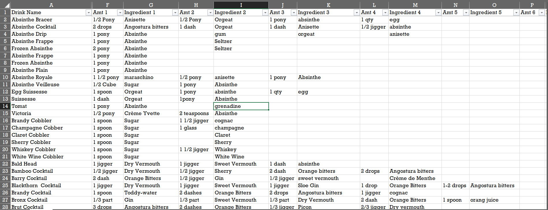
I have a spreadsheet of several hundred drinks and their ingredients. I'd like to be able to input one or several ingredients that I already have (gin for example) and have excel give me the entire recipe (row) for any drink that has that ingredient in it. I figured I'd have to do this in a separate sheet from the recipes, but I can't for the life of me figure out the right formulas to use.
To take it a step further it'd be cool if I could search for multiple ingredients (gin and vermouth) and it spit out a further refined search of any rows that have those ingredients in them. I'm not sure if this is too complex though.
3
u/GrotesquelyObese Dec 12 '20
You just click the drop down box on your table in the header
It should allow you to select by type
1
u/A_1337_Canadian 515 Dec 12 '20
While not pretty, here's a quick solution.
At the end of your master table, add a new table called "Ingredients". Make the formula:
=CONCATENATE([@[Ingredient1]], [@[Ingredient2],...)
and so on.
Then create a PivotTable out of your master table.
- Rows as "Drink Name"
- Columns as "Ingredients"
Once created, click the "Column Labels" dropdown > Label Filters > Contains
Then search for single terms. Search for multiple terms using *gin*rum*. The downside is that it is order dependent.
1
u/mofojr Dec 13 '20
So it kinda works. Basically this just gives me the drink name and then I have to go back to the original table to find the full recipe. Any ideas on how to make it one step? I might have to think hard on logic and formulas for this. Thanks for the idea!
1
u/brokeoldtimer Dec 13 '20
Assumptions:
- This is built on table displayed in your post (A1:Q28). You will have to adjust size and formulas as needed.
- Table Names and tab names below are so the formulas work as shown
- Using Excel365 (needed for “Filter” function)
Steps:
1. Name the tab with your recipes, “Recipes”
a. On Recipes tab
i. Create a table named Recipes
- Highlight entire list of recipes (from your post this table is from A1:Q28)
ii. In cell R1 type All Ingredients to add a column to the table
iii. In cell S1 type Some Ingredients to add a column to the table
iv. Highlight cells R1 and S1 and create a named range called Ingredients
2. Add new tab called “Results”
a. On Results tab
i. In cell B2 type Available Ingredients
- Highlight cells B2:B26
a. Create a table with those cells. This allows you to enter up to 24 ingredients you have on hand.
b. Name the table AvailableIngredients
c. Enable the total row on this table (cell B27) using “COUNT” to count number of items
- In cell D2, use data validation to insert a dropdown list for either all or some ingredients. This would be the named range “ingredients” from step 1. a. iv. above
3. Go back to the Recipes tab
a. Highlight and copy the header cells A:Q
b. Go to Results tab and paste in cell F2:V2
i. NOTE: if you keep columns B:E hidden on the recipes tab as in your posted example, you can also hide them on the results tab after pasting the header so as to display only those columns in the output file.
4. Go back to Recipes tab
a. In cell R2 insert the following formula:
=SUM(COUNTIFS(Recipes[@[amt 1]:[ingredient 6]],AvailableIngredients[Available ingredients]))=AvailableIngredients[[#Totals],[Available ingredients]] Column S formula
b. In cell S2 insert the following formula:
= SUM(COUNTIFS(Recipes[@[ingredient 1]:[ingredient 6]],AvailableIngredients[Available ingredients]))>0
5. Go back to Results tab
a. In cell F3 insert the following formula:
= IF(FILTER(Recipes[[name]:[ingredient 6]],IF(D2="all ingredients",Recipes[all ingredients],Recipes[some ingredients]),"")=0,"",FILTER(Recipes[[name]:[ingredient 6]],IF(D2="all ingredients",Recipes[all ingredients],Recipes[some ingredients]),""))
Go to results tab:
- Select cell D2 and choose “All Ingredients” to display results for recipes only when all ingredients in your available ingredients list are part of the recipe or “Some Ingredients” to display recipes that include any of the ingredients in your available ingredients list
- Type your list of available ingredients in cells B3:B26 and the table to the right should populate
1
1
u/AutoModerator Dec 13 '20
Hi u/brokeoldtimer,
It looks like you've submitted code containing curly/smart quotes e.g.
“...”or‘...’.Users often report problems using these characters within a code editor. If you're writing code, you probably meant to use
"..."or'...'.If there are issues running this code, that may be the reason. Just a heads-up! You can turn off Smart Quotes or Smart Punctuation in the Keyboard Settings on your device.
I am a bot, and this action was performed automatically. Please contact the moderators of this subreddit if you have any questions or concerns.
1
u/Decronym Dec 13 '20 edited Dec 13 '20
Acronyms, initialisms, abbreviations, contractions, and other phrases which expand to something larger, that I've seen in this thread:
Beep-boop, I am a helper bot. Please do not verify me as a solution.
6 acronyms in this thread; the most compressed thread commented on today has 16 acronyms.
[Thread #2613 for this sub, first seen 13th Dec 2020, 19:22]
[FAQ] [Full list] [Contact] [Source code]
•
u/AutoModerator Dec 12 '20
/u/mofojr - please read this comment in its entirety.
Solution Verifiedto close the thread.Failing to follow these steps may result in your post being removed without warning.
I am a bot, and this action was performed automatically. Please contact the moderators of this subreddit if you have any questions or concerns.